1. Schottky diode 1. Schottky diode

1.1  C/V and I/V curves

1.1.1  C/V curve

The capacitance C of a Schottky contact with the area F is:

C = eF
W
(1.1)
W is the width of the space charge region, e = e0 er the dielectric constant.

For a homogenous distribution of the shallow concentration NS yields the integration of the Poisson equation to:

W =   æ
 ú
Ö

2e(U+UD)
qNS
 
(1.2)
q is the elementary charge, UD the diffusion voltage and U an external voltage.

From this follows:

C = F   æ
 ú
Ö

eqNS
2(U+UD)
 
(1.3)
The linear form of this equation is:
1
C2
= 2
eF2qNS
(U+UD)
(1.4)
By the linear regression you get from the slope NS and from the intersection UD. You can calculate the barrier height fB from UD by the following equation:
qfB
=
qUD + (EC-EF)
(1.5)
EC-EF
=
kTln( NC
NS
)
(1.6)

1.1.2  Pulse capacitance CP

The reverse bias capacitance will every time measured. The capacitance during the pulse can be measured or calculated. In the second case you get this value from:

CP
=
F   æ
 ú
Ö

eqNS
2(UP+UD)
 
(1.7)
UD
=
F2eqNS
2CR2
- UR
(1.8)
NS you get from the C/V-curve. This equation takes into acconut only a temperature dependance of UD but not of NS.

1.1.3  Shallow doping profiles

The following equations are the 4 possibilities in the software:

NS(x)
=
2C2
qeF2
(U+UD)
(1.9)
NS(x)
=
2
qeF2
(
d 1
C2

dU
)-1
(1.10)
NS(x)
=
_
N
 

S 
(x) + 1
2
x
d _
N
 

S 
(x)

dx
    with _
N
 

S 
from (1.9)
(1.11)
NS(x)
=
_
N
 

S 
(x) + 1
2
x
d _
N
 

S 
(x)

dx
    with _
N
 

S 
from (1.10)  
(1.12)
The standard method is 2, but from the physics the method 4 is the best.

Another expression for eqn. (1.10) is:

NS(x) = - C3
qeF2
dU
dC
(1.13)
The depth x you can calculate by:
x = eF
C
(1.14)

1.1.4  I/V curve

I(U) = IS æ
ç
è
exp æ
ç
è
qU
nkT
ö
÷
ø
-1 ö
÷
ø
(1.15)
n is the ideality-factor or n-factor, in the software called n-fac. The saturation current is:
IS = F A* T2 exp æ
ç
è
-qfB
kT
ö
÷
ø
(1.16)
A* is the Richardson constant corrected by the effective mass:
A* = A m*n
me
(1.17)
m*n is the effective mass for electrons, me is the electron mass.

If qU >> nkT, then follows:

I(U) = IS exp æ
ç
è
qU
nkT
ö
÷
ø
(1.18)
The linear form of this equation is:
ln(I) = ln(IS) + q
nkT
U
(1.19)
By the linear regression you get from the slope n and from the intersection IS. With eqn. (1.16) you can calculate the barrier height fB:
qfB = kT ln æ
ç
è
F A* T2
IS
ö
÷
ø
(1.20)
From fB you can calulate UD by eqn. (1.5).

1.1.5  Richardson plot

JS = IS
F
(1.21)
To get fB from the eqns. above you must know the Richardson constant. You can calculate fB without A* by the Richardson plot:
ln æ
ç
è
JS
T2
ö
÷
ø
= ln(A*) - qfB
k
1
T
(1.22)
By the linear regression you get from the slope fB and from the intersection A*. This plot you can make in the C/V- I/V-module, menu 2.1.1. For this you must measure the I/V-curves at different temperatures and make the evaluation in menu 2.6.5, so that you get JS resp. IS for different temperatures.

In the tempscan evaluation module, menu 6.4.5.5.4, there is a plot similiar to the Richardson plot:

ln æ
ç
è
JR
T2
ö
÷
ø
= ln(A*) - qfB
k
1
T
(1.23)
Note that in this plot you have the reverse bias current and not the saturation current as necessary for the true Richardson plot. So your data obtained by this evaluation are not the correct values although they was called as in the true Richardson plot!

1.2  DLTS-transients

Fig. 1.1: Band diagram of a Schottky-diode

1.2.1  Transients

For NT << NS is the following equation valid for the capacitance DLTS method (C-DLTS):

C(t)
=
CR - DC exp(-t/te)
(1.24)
DC
=
CR NT
2NS
LR2-LP2
WR2
(1.25)
LR,P
=
WR,P - l
(1.26)
The index R resp. P means the value at reverse bias UR resp. at pulse voltage UP. DC is the transient amplitude. The equation above contains the lambda shift.

The distance l = W-L is voltage independent at a homogenous distribution:

l =   æ
 ú
Ö

2e(EF-ET)0
q2 n0
 
(1.27)
(EF-ET)0 is the distance between trap- und Fermi level in the undisturbed semi conductor. The program takes here your energy value from the Arrhenius plot or from the sample parameters.

For voltage transients (U-DLTS) is valid:

U(t)
=
UR - DU exp(-t/te)
(1.28)
DU
=
qeF2 NT
2CR2
LR2-LP2
WR2
(1.29)
For the reverse bias is valid:
UR = q
2e
(NS-NT)WR2 + q
2e
NT LR2-UD
(1.30)
IF you select the reverse bias and the pulse voltage in such kind that LP » 0 and l << WR, so are the amplitudes approximately:
DC
»
CR NT
2NS
(1.31)
DU
»
qeF2
2CR2
NT
(1.32)
For the current transient you get in this case:
I(t) - IR = 1
2
q F WR NT 1
te
exp(-t/te)
(1.33)

In the software the normal plots for transients are CR-C(t), UR+U(t) for n-type, UR-U(t) for p-type and I(t)-IR.

1.2.2  Trap concentration

From eqn. (1.25) and (1.29) you get the exact trap concentration:

NT
=
2 NS DC
CR
WR2
LR2-LP2
   for C-DLTS
(1.34)
NT
=
DU 2CR2
qeF2
WR2
LR2-LP2
   for U-DLTS
(1.35)
In the program these values will be called NTe or exact trap concentration, except in menu 4.1.4. There the plots of doping profiles are called NT(x), but are calulated by the exact equations.

For the approximation after eqn. (1.31) and (1.32) you get:

NT
=
2 NS DC
CR
   for C-DLTS
(1.36)
NT
=
DU 2CR2
qeF2
   for U-DLTS
(1.37)
In the program these values will be called NT, trap concentration or approximated trap concentration. This is the standard calculation of NT in the literature or with standard DLTS-systems.

1.2.3  Analysis of NT-doping profiles

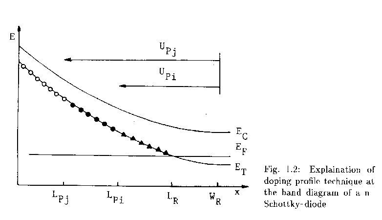
At the U-DLTS-method you get from the integration of the Poisson equation for the voltage transient Ui(t) with the pulse voltage UPi:

Ui(t)-UR
=
- q
e
LR
ó
õ
LPi 
xNT(x) exp(-t/te) dx
(1.38)
UR
=
q
e
æ
ç
è
NSWR2
2
- WR
ó
õ
LR 
xNT(x) dx ö
÷
ø
-UD
(1.39)
For the difference of two transients with pulse voltages UPj and UPi are only the traps between LPj and LPi relevant for the signal:
Uji(t) : = Uj(t)-Ui(t) = - q
e
LPi
ó
õ
LPj 
xNT(x)exp(-t/te) dx
(1.40)
With the definition of a medium trap concentration you get the following approximation:
Uji(t)
»
- q
2e
(LPi2-LPj2) _
N
 

T 
(xji) exp(-t/te)
(1.41)
xji
: =
LPj+LPi
2
(1.42)
The amplitude of charge is then:
DUji = - q
2e
(LPi2-LPj2) _
N
 

T 
(xji)
(1.43)
You can calulate the medium trap concantration following:
_
N
 

T 
(xji) = - 2e
q
DUji
(LPi2-LPj2)
(1.44)
For the C-DLTS-method you get approximately:
_
N
 

T 
(xji) = 2NSe2F2
CR3
DCji
(LPi2-LPj2)
(1.45)
DCji is the amplitude difference of the two capacitance transients.

For this technique you must make a measurement in 4.7.2.1 and a evaluation in 4.1.4.3. In menu 4.7.4.1 you get a NT(x)-plot without building of differences. This yields normally to a big error because you have in this case a very brought xRi-range.

This technique is analog to technique (a). The disadvantage of this method is that the relevant charges are at the intersection Fermi/trap level. You can make this measurement in 4.7.2.2.

A profile analysis is also possible without building of differences:

_
N
 

T 
(xi)
=
2 NS DCi
CRi
WRi2
LRi2-LPi2
   for C-DLTS
(1.46)
_
N
 

T 
(xi)
=
DU 2CRi2
qeF2
WRi2
LRi2-LPi2
   for U-DLTS
(1.47)
For this technique you must make a measurement in 4.7.2.3 and a evaluation in 4.1.4.1.

1.3  Kinetic

1.3.1  Emission

For the with electrons filled traps nTe is valid during the emission process:

nTe(t)
=
NT exp æ
ç
è
- t
te
ö
÷
ø
(1.48)
with        te
=
æ
ç
è
sn vth,n Xn NC exp æ
ç
è
- EC-ET
kT
ö
÷
ø
ö
÷
ø
-1

 
(1.49)
NT is the trap concentration, Xn the entropy factor, sn the capture cross section for electrons and te the emission time constant. In the software te is called time constant, emission time constant, tau or tau_e.

The emission rate is the reziproke value of the emission time constant:

en = 1/te
(1.50)
You get the thermal velocity vth,n and the state density NC from:
vth,n
=
  æ
 ú
Ö

3kT
m*n
 
   
(1.51)
NC
=
2 æ
ç
è
2 pm*n kT
h2
ö
÷
ø
3/2

 
(1.52)
m*n is the effective mass for electrons. Transforming of eqn. (1.49) yields to the Arrhenius-equation:
ln(te vth,n NC) = EC-ET
k
1
T
-ln(Xn sn)
(1.53)
By the linear regression you get from the slope EC-ET and from the intersection the product sn Xn. This equation contains the T2-correction.

In the program sn Xn will called as capture cross section, sigma or sig. In the library part of the software the name is Sigma Arrhenius, Sigma-Arrh or sig-Arrh.

One of the text possiblity for the y-axis of the Arrhenius plot is ln(tau*T2*C).
C means here all constants of vth,n NC except of the temperature. So C is [(vth,n NC)/( T2)] for electrons and [(vth,p NV)/( T2)] for holes. tau of the y-axis-text is the emission time constant te.

1.3.2  Capture

For the with electrons filled traps nTc is valid during the capture process:

nTc(t)
=
NT æ
ç
è
1-exp æ
ç
è
- t
tc
ö
÷
ø
ö
÷
ø
(1.54)
with        tc
=
1
sn vth,n n0
(1.55)
tc is the capture time constant. In the software tc is called capture time constant or tau_c. Following is valid:
cn
=
sn vth,n n0 = 1/tc     capture rate
(1.56)
c¢n
=
sn vth,n     capture coefficient
(1.57)
n0
=
NC exp æ
ç
è
- EC-EF
kT
ö
÷
ø
(1.58)
The program takes NS as n0.

In the program sn will called as capture_c cross section, sigma_c or sigmaC. In the library part of the software the name is Sigma Capture or sig-Capt.